How to Tackle Complex Math Assignments Using the Mean Value Theorem

When tackling mathematics assignments, particularly those involving the Mean Value Theorem (MVT), it's crucial to understand both the theoretical aspects and how to apply them in practical problems. For many university students, concepts like the Mean Value Theorem can be challenging, especially in calculus. However, breaking down these concepts can make them much easier to comprehend and apply. In this blog, we focus on two major types of Mean Value Theorems: the Lagrange Mean Value Theorem (Lagrange MVT) and the Generalized Mean Value Theorem, often called the Cauchy Mean Value Theorem. Both of these are foundational in calculus, offering a method to relate the derivative of a function to the average rate of change over an interval.
The Lagrange MVT states that for a continuous and differentiable function, there exists at least one point where the instantaneous rate of change (the derivative) equals the average rate of change over an interval. On the other hand, the Cauchy MVT generalizes this concept by involving two functions and their derivatives. Understanding these theorems and practicing with examples will help to solve their math assignment much more manageable. With a solid grasp of the core concepts, you’ll be able to approach MVT problems with confidence and ease.

What is the Mean Value Theorem?
The Mean Value Theorem (MVT) is a fundamental concept in calculus that provides a relationship between a function’s average rate of change and its instantaneous rate of change. More precisely, the theorem states that for a continuous function that is differentiable over a certain interval, there exists at least one point where the derivative of the function equals the average rate of change over that interval.
Mathematically, the MVT states:
If a function f is continuous on the closed interval [a, b] and differentiable on the open interval (a, b), then there exists a point c in (a, b) such that:
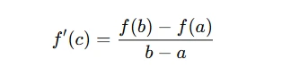
This equation means that there’s at least one point where the slope of the tangent to the function is equal to the slope of the secant line connecting the points (a, f(a)) and (b, f(b)).
How to Apply MVT in Your Assignments?
When solving problems related to the Mean Value Theorem in your assignments, the first step is ensuring the function satisfies the conditions of the theorem. For example, ensure the function is continuous on the closed interval and differentiable on the open interval. These conditions are necessary for you to apply the MVT correctly.
Let’s take a simple example:
Suppose f(x)=x2 on the interval [1, 3]. The function is continuous and differentiable on this interval, so you can apply the Mean Value Theorem.
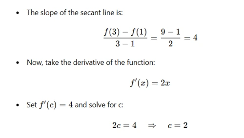
So, at x = 2, the slope of the tangent line is 4, which matches the slope of the secant line.
Challenges You Might Face
While the Mean Value Theorem may seem straightforward, several challenges could arise when applying it:
- Verifying Continuity and Differentiability:
- Geometric Interpretation:
- Solving for c:
You must check if the function is continuous on the closed interval and differentiable on the open interval. Many functions may look continuous but fail to meet these conditions at some point. For example, piecewise functions can often create confusion, as they may not be differentiable at the point where the pieces meet.
It’s often helpful to visualize the problem geometrically. You should be comfortable sketching the graph of the function and identifying the secant line, as well as the tangent lines. This visual representation helps you understand why there must be at least one point where the instantaneous rate of change matches the average rate of change.
Solving for c, the point where the instantaneous rate of change matches the average rate of change, can sometimes involve more complex equations. Be cautious with algebraic manipulation, and always double-check your calculations.
Lagrange Mean Value Theorem: A Generalization
The Lagrange Mean Value Theorem (Lagrange MVT) is an extension of the Rolle’s Theorem and the classical MVT. It provides a slightly more generalized result. While the Mean Value Theorem requires that the function be equal at the endpoints of the interval, the Lagrange MVT does not have this condition. The Lagrange MVT is applicable to a wider range of functions.
The theorem states:
If a function f is continuous on the closed interval [a, b] and differentiable on the open interval (a, b), then there exists at least one point c in (a, b) such that:
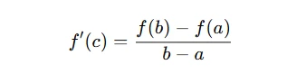
This result is similar to the MVT, but it does not require that f(a)=f(b). Instead, the Lagrange MVT allows for any continuous and differentiable function, even if the values at the endpoints are different.
Geometric Interpretation of the Lagrange MVT
Geometrically, the Lagrange MVT states that if you draw a secant line between the points (a, f(a)) and (b, f(b)), there will be at least one point c in (a, b) where the tangent line to the curve at that point is parallel to the secant line.
In simpler terms, if you connect the two points on the curve, there’s at least one point along the curve where the slope of the curve is the same as the slope of the secant line joining the endpoints.
The Proof of Lagrange Mean Value Theorem
To prove the Lagrange MVT, we use Rolle’s Theorem. The idea is to define a new function φ(x)=f(x)−(f(b)−f(a)/b−a)x, which is a linear transformation of f(x). Applying Rolle’s Theorem to this new function shows that there exists a point where the derivative is zero, which implies that the slope of the tangent line at that point matches the slope of the secant line.
The Cauchy Mean Value Theorem: Generalized Case
The Cauchy Mean Value Theorem, also known as the Generalized Mean Value Theorem, extends the concept further. Instead of applying to a single function, this theorem applies to two functions, f(x) and g(x), and it relates their rates of change at a particular point.
The Cauchy Mean Value Theorem states:
If f(x) and g(x) are continuous on the closed interval [a, b], differentiable on the open interval (a, b), and g'(x) does not vanish anywhere in the interval, then there exists a point c in (a, b) such that:
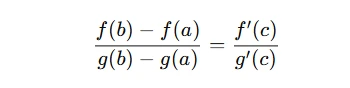
This theorem allows us to compare the rates of change of two different functions at a particular point. It is a powerful tool in problems involving two functions with related rates.
How to Use the Cauchy Mean Value Theorem in Assignments?
To apply the Cauchy MVT in your assignments, follow similar steps as in the previous examples, but with two functions involved. Make sure both functions meet the continuity and differentiability conditions. Often, you’ll be asked to find a ratio of derivatives at some point, and using this theorem will simplify the problem.
For example, if you have two functions f(x)=x2and g(x)=x, you can use the Cauchy Mean Value Theorem to find the point where their rates of change are proportional.
Conclusion
Understanding the Mean Value Theorem, Lagrange Mean Value Theorem, and Cauchy Mean Value Theorem is crucial for solving calculus problems, especially when working on assignments. By grasping the geometric interpretations, conditions, and application techniques for each theorem, you’ll be able to solve problems with confidence.
However, there are some common challenges to keep in mind, such as verifying the conditions of the theorems, understanding the geometric interpretations, and solving for unknowns. By practicing regularly and thoroughly understanding the theory, you’ll develop the skills needed to approach these problems effectively.
For your assignments, always ensure you understand the conditions for applying these theorems and take the time to visualize the problem geometrically. This will not only help you solve the problems but also give you a deeper understanding of how calculus operates in real-world scenarios.